|
|
A variety of factors conspire to make high-resolution high-dynamic-range astrophotography a difficult task: the amount of incident light at Earth from objects tens or hundreds of light years away is very small, necessitating very large aperture lens systems. The celestial objects typically subtend small visual angles compared to terrestrial subjects, requiring long focal lengths (further confounding the aperture size problem). The Earth's atmosphere is often highly turbulent (or even cloudy), leading to difficulty creating a well-focused image from the ground; and Earth's axial rotation causes movement of the subjects. In this study, we focus on the last of these problems. The Earth's rotation about its axis causes astronomical objects to appear to move across the sky. Even at relatively low magnifications, astronomical images are highly susceptible to motion blur. In theory the motion blur is quite predictable, but in practice it is influenced by many other factors such as vibration and atmospherics. |
 |
It is relatively easy to calculate the exact amount of blur which will occur in a given exposure.
The field of view of a lens is given by:  .
The rotation of the Earth is approximately
.
The rotation of the Earth is approximately  or about
  .
Thus, the length of a blur streak as a fraction of the frame, can be found as:
.
Thus, the length of a blur streak as a fraction of the frame, can be found as:
 where exposure time is measured in seconds.
Consider some relatively common numbers for standard commercial telescopes and cameras:
where exposure time is measured in seconds.
Consider some relatively common numbers for standard commercial telescopes and cameras:
Plugging these values into the above equation, we find that the blur streaks will be approximately 1/6th of the diagonal length of the frame.
In terms of images, motion blur obeys a simple mathematical model. If we assume that the subject and observer do not change positions (a relatively good assumption considering the relative distances involved), the apparent motion of the subject is precisely the actual angular motion of the observer. This may be described by a path across the blurred image which any source point follows during the duration of the exposure. The value of the observed image will then be the average value along that path of the latent image which would have been observed in the absense of motion blur, i.e. if the orientation of the camera with respect to the subject had remained constant throughout the exposure. In other words, the observed image is the (two-dimensional) convolution of the path of motion with the latent image [3]. We define our task to be recovering the latent image given the observed image. We further denote the graph of the path of motion as the point spread function of the motion blur.
We can express any two dimensional image convolution by a point spread function as: ![]() . In order to recover the latent image, we must determine the point spread function, and find an appropriate means of reversing the convolution, that is, deconvolving the image.
. In order to recover the latent image, we must determine the point spread function, and find an appropriate means of reversing the convolution, that is, deconvolving the image.
|
Astronomical photographers generally solve the motion blur problem by using extremely high quality tracking telescope mounts. These mounts use precisely machined gears and high accuracy motors to follow astronomical objects. These mounts are often augmented by special CCD "autoguiders" or manual human guiders that use bright celestial objects (usually stars) as reference points. These guiders command the telescope's motors to make slight corrections in their paths. Additional error due to instantenous atmospheric turblence, vibrations, and small mechanical defects can be reduced through the use of adaptive optics systems which use small, rapidly moving mirrors to keep a single point at the center of the image at all times. Needless to say, these techniques are expensive and require enormous amounts time and effort to setup, learn and perfect. |
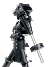 Losmandy HGM Titan: http://www.losmandy.com/ |
The problem of recovering a latent image from a convolved one (termed deconvolution) is well-studied in the literature of digital photography. Assuming knowledge of the point spread function, there are several common techniques. That is, we wish to compute: 
The deconvolution problem has been extensively studied due to its many applications in a variety of areas. Indeed, the Space Telescope Science Institute held a conference on image restoration for data from the Hubble Space Telescope in 1993 (http://www.stsci.edu/stsci/meetings/irw/) in which several new deconvolution methods were proposed. The deconvolution literature is thus extremely extensive and a proper survey is far beyond the scope of our project. We will concentrate on several of the most commonly used method and weigh their strengths and weaknesses.
|
The most straight-forward procedure is to perform a formally exact inverse of convolution. Since convolution is equivalent to pointwise multiplication in the frequency domain, deconvolution can be accomplished by pointwise division in the frequency domain. Unfortunately, this technique very rarely yields useful results in practice. There are two problems. First, the observed image is not exactly the convolution of the latent image with the point spread function; this is due to the introduction of noise by the imperfect sensors in real-world cameras. In practice the magnitude of the noise may be quite large, depending on imaging conditions. Second, in the event that the frequency domain representation of the point spread function contains zeros, division is meaningless and it is impossible to recover a frequency-domain representation of the deconvolved image. The second issue is badly compounded by limited numerical precision in processing and capture. As one can tell from the adjacent image, the results of this trivial deconvolution typically contain an overwhelming amount of noise and are not of much use. |
 Frequency Domain Division Deconvolution (Beehive Cluster) |
Despite the many problems with this method, it does have the advantage that it extremely fast. It involves just three fast fourier transforms and can be completed in seconds on modern processors for images with megapixel sizes.
FFT Deconvolution: 
There are many potential tweaks one can attempt with the frequency domain division deconvolution algorithm to avoid zeros in the point spread function and produce better images. One can introduce noise to the point spread function to give it non-zero values in the frequency domain. Indeed, during our work with frequency domain deconvolution, we tried introducing a variety of different noise functions including gaussian noise, random noise over a small interval and noise synthesized from noisy but unoccupied pieces of the image. One can also apply certain filters to attempt to remove particularly noisy portions of the frequency domain after division. For instance, one can take advantage of the fact that the latent astronomical image consists principally of high frequencies and use a high pass filter to remove low frequency noise.
Others have dabbled with various tricks for removing zeros. Reiter [2] proposes a modification to this technique which reduces the problem somewhat. In his method, the frequency spectrum of the point spread function is modified by a simple formula retaining the general shape of the spectrum but smoothly replacing all zeros by a relatively small constant. He offers no explanation for his idea, but claims that it produces usable results. However, substantial artifacts remain.
The frequency domain division technique is very fast but does not produce very high quality images. Fortunately it is possible to do deconvolution without division in the frequency domain. Another important class of deconvolution algorithms assume a model in which the observed image is a the sum of a perfect convolution with random noise from some particular distribution. One such algorithm was independently conceived by W.H. Richardson (1972) and L.B. Lucy (1974) [6].
The Lucy-Richardson algorithm is an iterative algorithm which is derived from Bayes' theorem. Starting with a guess for the original image, the Lucy-Richardson algorithm updates its guess on each iteration so it tends toward the latent image. In theory, the longer the algorithm is iterated, the closer it comes to converging to the latent image. The algorithm uses the update rule:  where i,j and k represent pixels in the image.
The algorithm as stated above is not efficiently computable; it requires iteration over all of the pixels of the image in three levels of nested loops for each iteration of the algorithm. Fortunately, the algorithm can be sped up dramatically by using frequency domain convolution in place of the inner summations. Although the algorithm remains quite slow, it is at least feasible to compute it on images in the several megapixel range, provided that the user is willing to wait tens of minutes.
Although Lucy-Richardson calls for a division, it is not a frequency domain division, so the corresponding noise amplification is very localized. As a result, the images it produces do not exhibit the periodic noise and ghostly streaks that show up when frequency domain division is used.
We also attempted to do deconvolution using Wiener filters, which are supplied in Matlab. Wiener filters are supposed to minimize the squared error of inverse filtering and noise smoothing. Perhaps because we lacked a good noise model, our results were not acceptable. [1]
From our experience most applications of deconvolution are to removing misfocus or lens aberations. To this end, lens manufacturers typically can provide a PSF to researchers. We have seen very little research on identifying PSF's for motion blur.
Reiter [2] notes that it is possible to determine motion blur directionality by observing the parts of the captured image corresponding to high-contrast sources. His method, however, is relatively primitive: "by experimenting, we identified a line segment that corresponded to the motion blur. Notice that the extent of motion blur can be estimated by the barely visible edges of the gasoline cap cover in the blurred image." His work is also not specifically concerned with astrophotography. Similar techniques are discussed in the documentation for the Matlab Image Toolbox.
We explored three different methods for estimating the point spread function of the motion blur.
|
This technique relies on the theory that at any reasonable magnification, a star should appear to an Earth-bound observer as a point source. This is because stars are so distant; even Proxima Centauri, the closest star to Earth, is 4.22 light years, or 4E16 meters away. Normal stars are 7E7 meters in diameter, so the tangent of the angle subtended is 1.75E-9. That's roughly 1E-7 degrees. For a 2800mm telescope, the field of view is 0.7 degrees, so a star covers roughly a millionth of the image (which is less than a hundredth of a pixel on most cameras). Because a star appears as a point source, the observed image of a star should be precisely the point spread function of the optical process. Based on this idea, we proposed extracting parts of the image around star trails and using them unchanged as point spread functions for the deconvolution algorithms above. | 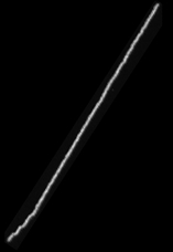 |
|
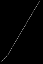
The "image chunk PSF" idea has two important shortcomings. First, the image captured contains noise in addition to the image of the stars, and any chunk extracted around a particular star trail is likely to contain (faint) trails of other stars as well. Second, the method approximates the PSF of the entire optical process rather than just that of the motion blur. While removing all of the blur would be an appealing result, it is much less numerically feasible. The blur in the motion direction is sharp and contains many high frequencies, improving the conditioning of the numerics. By contrast, the blur in the perpendicular direction is Gaussian and therefore deficient in high frequencies. Another obvious method is to measure the length and angle of a star trail, and construct a PSF containing a simple straight line with that length and angle. Such a PSF contains no noise or extraneous trails, and only models the blur resulting from motion; it does not model the blur resulting from focus problems or atmospheric turbulence. As a result, deconvolution with this PSF is more numerically stable. | 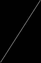 |
The principal component of motion during an exposure is the angular motion of the Earth, which can be approximated as a straight or gently curved line segment through the blurred image. However, significant variations may be introduced by seismic vibrations of the observation location or by temporal fluctuations in the atmospheric density (and hence index of refraction) along the line of sight. Any deviation from an exact straight line will produce ghosting in the deconvolved image if we use the Straight Line estimate for the PSF as above.
Note that if the overall optical transparency of the atmosphere changes over the course of the exposure, the observed image will not simply be the convolution of the path of motion with the latent image. Rather, each value in the observed image will be a weighted average of values from the latent image, where the weighting is by the optical transparency. We can still pose the problem as a deconvolution, however; we simply include the optical transparency as a factor in the graph of the motion path, obtaining a slightly fancier point spread function which accounts for both the path of the point source and changes in its luminosity. To contrast, the straight line point spread function assumes a linear path and does not account for changes in luminosity.
For simplicity assume the direction of blur is roughly along the X axis. Given an image containing just one streak, we developed the following iterative algorithm to estimate the path of motion f(x), the optical transparency m(x), and the cross-sectional blur g(x):
ALGORITHM estimatePath

FOR EACH x
  m(x) := norm of column x of the streak
  rescale column x to have norm 1
END

g := central column of the streak
f := 0 for all x

REPEAT UNTIL f, g converge
  FOR EACH x
    f(x) := the value of y which minimizes
      the sum of squared errors between
      g shifted by y and the x'th column
      of the streak
  END

  FOR EACH y
    g(y) := average over all x of streak(x, y+f(x))
  END
END
|  |
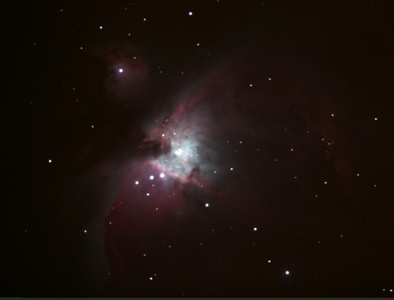
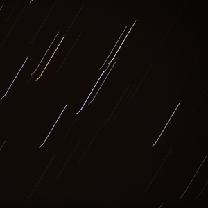
We used a Celestron NexStar 11GPS 2800mm Schmidt-Cassegrain telescope and a Canon Digital Rebel XT digital SLR camera to capture several astronomical images with tracking turned off. For comparison, we also captured tracked images. The images displayed below are of the Beehive Star Cluster (Messier Object #44) and the Orion Nebula (Messier Object #42). They were taken with 30 second exposures at ISO 1600. A reducer corrector was used to give the telescope an effective focal length 1800 mm. In order to meet reasonable time requirements, we cropped and downsampled images to a resolution of 1024x1024 from 3456x2304. The color channels were extracted from RAW images and kept in 16 bit image formats in order to exploit the full dynamic range of the Digital Rebel's 12 bit Analog/Digital converter. All processing was done with 64 bit floating point arithmetic.
We implemented each of the methods of identifying a point spread function discussed above. The results we show were deconvolved using the Lucy-Richardson algorithm, but in principle any of the deconvolution algorithms mentioned in Section 2 would have worked.
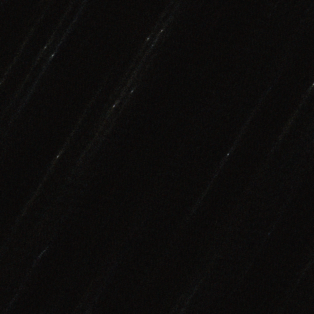
| Original (Beehive Cluster) | 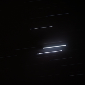 Original (Orion Nebula) |
On the left, our photograph of the Beehive cluster exhibits some early vibration that is roughly perpendicular to the direction of motion. We believe that the vibration may have been caused by the camera's mirror flipping or perhaps the shutter. This nonlinearity is absent from our image of the Orion Nebula. Neither of these images has been rotated; the differing directions of stellar motion are due to them having been taken in different areas of the sky.
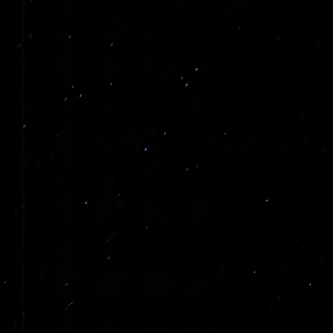 Image Chunk PSF Deconvolution (Beehive Cluster) | 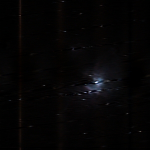 Image Chunk PSF Deconvolution (Orion Nebula) |
This method worked well for the isolated star case on the left, but produced very blury results for the nebula on the right. These problems are probably partially due misfocus, certain telescope aberrations and CCD problems which may have caused parts of the streak to be overexposed and spread to surrounding pixels. These problems lead to a gaussian fall off in intensity in the direction perpendicular to the streak which is difficult to rectify through deconvolution. Also, it is possible that aperiodic camera noise in readout and certain "bad pixels" caused the some inconsistancies in the streak.
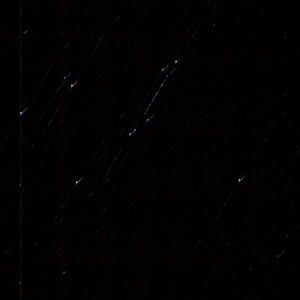 Straight Line PSF Deconvolution (Beehive Cluster) | 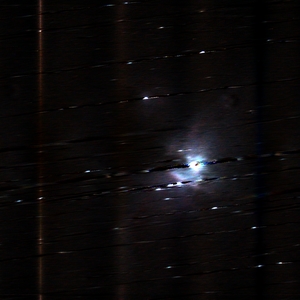 Straight Line PSF Deconvolution (Orion Nebula) |
Many motion blur correction techniques including those suggested in the Matlab documentation, the commericial product ImageLab, and Rieter[2] suggest using a straight line to approximate motion blur. As one can see from the above images, this technique only works well when motion can be very accurately approximated as straight line. The early non-linear motion in the M44 image was sufficient to cause significant ghosting. However, the Orion Nebula looks considerably better than it did with the image chunk technique. The PSF is an anti-aliased line which is approximately one pixel in width and thus does not attempt to correct for any cross-sectional blur which was present in the image chunk technique. As previously mentioned, correcting for gaussian focal blur (or gaussian blooming) is a difficult problem and may actually introduce additional artifacts.
 Motion Estimation PSF Deconvolution (Beehive Cluster) |  Motion Estimation PSF Deconvolution (Orion Nebula) |
|
Our motion estimation algorithm attempts to attain the "best of both worlds." It ignores the cross-sectional gaussian blur while very accurately producing a path through the image. We actually construct the path with subpixel accuracy by bicubically rescaling the input up by a factor of 8x before applying the motion estimation algorithm. The rational for this is that the graylevels present in the original image define a curve which may not be best matched at an integral pixel boundary. The motion estimation method performs visibly better than the bad cases of the other two methods, and not worse than the good cases. In fact in the high resolution images this method looks somewhat better than the good cases too. We can also trivially extract cross-sectional diagrams and intensity curves as part of this method. The adjacent image shows (from top to bottom): the original star trail from a chunk of the image, the path our motion tracking algorithm found, the intensity of the streak as computed using the norm of each individual cross-section, and the estimated intensity distribution of the cross-section. Note that the motion tracking path we compute, which we use as a point spread function, very accurately fits the original star trail. Also note that the average cross-section of the original observed star trail very precisely fits the expected gaussian model. We do find the intensity variations to be quite large. We attribute these fluctuations to a combination of vibrations and atmospheric turbulence. As this is an absolute scale and changes are registered over several pixels, we do not believe the observed fluctuations can be the result of noise in the camera. |
 Motion Estimation Graphs |
Our method of extracting a point spread function based on estimating an exact path of motion from a star trail qualitatively outperformed both the chunk-based point spread function and the straight-line point spread function. When combined with a noise-resistant deconvolution algorithm such as Lucy-Richardson iteration, this technique is a robust high-quality motion blur removal system for astrophotographic images.
There are several interesting directions for future research on motion blur removal. In images containing multiple star trails, it is possible that combining path information from several trails could result in a still better estimate for the point spread function of the process. It may also be possible to apply some kind of filter to reconstruct the "dead" areas behind saturated star trails to provide a more visually pleasing (if not completely accurate) image.
One interesting possibility that arises from this work is a new method for taking high dynamic range images. In the case of a high magnitude source which is relatively small in an otherwise low-magnitude image, intentional motion blur can be used to spread the incoming light from the bright source over a larger area, thereby allowing a longer exposure (and hence more information content) to be captured. Upon reconstruction, an image with a dynamic range significantly higher than a non-blurred image could be produced.